
Use the swisstopo API to get a profile of altitudes with the function get_swisstopo_elevation_profile by passing coordinates aka “Rechtswert” and “Hochwert” as array/list (any iterable should do). The gist on GitHub should always be the most up-to-date version
Python
defget_swisstopo_elevation_profile(coords, # a path (2+ points in the form)kind='csv',# three heights are available for JSON# COMB, DTM2, DTM25which='COMB',asnumpy=True,quiet=True,opts={"sr": None,"nb_points": None,"offset": None,"distinct_points": True,"callback": None, } ):""" Call the swisstopo API for altitude data along a path. Pass in a list or array of coordinates in EPSG 2056 (LV95) or 21781 (LV03) to get altitude values along the provided path. For options see keywords or parameters of call via swisstopo API. Parameters ---------- coords : list or numpy array The coordinates in either EPSG 2056 (LV95) or EPSG 21781 (LV03). kind : str, optional Which API backend should be queried. Available are json and csv. If none of these are passed properly, fallback is csv. The default is 'csv' (easier structure to parse). which: str If kind is json, three altitude values are available, DTM2, DTM25 and COMB(INATION). asnumpy : bool, optional Whether to return a numpy array. The default is True. quiet : bool, optional Whether to quiet the output (True) or not. The default is True. opts: dict Further keywords than can be passed to the API call, see https://api3.geo.admin.ch/services/sdiservices.html#profile Returns ------- list or numpy array The returned points, in the form of distance along path, altitude, coordinates. """import requestsimport numpy as npiflen(coords) >5000:print('Warning, number of coordinates exceeds swisstopo API''max number of points, reduce coords beforehand.')return np.asarray([]) if asnumpy else [] payload ='geom={"type":"LineString","coordinates":[' payload +=','.join([f"[{coord[0]},{coord[1]}]"for coord in coords]) payload +=']' opts =','.join(['"'+str(key)+'"'+':'+'"'+str(opt)+'"'for key, opt in opts.items()if opt isnotNone])if opts: payload +=','+ opts payload +='}' kind = kind.lower()if kind.lower() notin ['csv', 'json']:ifnot quiet:print('Only csv or json can be chosen, autoselecting csv') kind ='csv' baseurl ="https://api3.geo.admin.ch/rest/services/profile."+ kindtry: profile = requests.get(baseurl, params=payload)exceptConnectionError:ifnot quiet:print('Connection timeout')return np.asarray([]) if asnumpy else []if profile.ok:ifnot quiet:print('Success')else:ifnot quiet:print('Failed')if kind =='csv': profile = profile.text.split('\r\n')# Distance, Altitude, Easting, Northing -> not needed# header = profile[0] profile =list(map(lambdax: [float(j.strip('"'))for j in x.split(';')], profile[1:-1]))elif kind =='json': profile = [[p['dist'], p['alts'][which], p['easting'], p['northing']]for p in profile.json()]if asnumpy: profile = np.asarray(profile)return profileif__name__=='__main__':# straightforward example usage rw=[2611025.0, 2620975.0, 2633725.0] hw=[1266400.0, 1256750.0, 1250000.0] profile = get_swisstopo_elevation_profile(list(zip(rw, hw)))import matplotlib.pyplot as plt plt.fill_between(profile[:,0], profile[:,1], facecolor='grey',edgecolor='k',alpha=0.8) plt.ylim(min(profile[:,1]), None)
Background/motivation
For the CLOUDLAB project we regularly get forecasts that contain a profile at the bottom of the figure from MeteoSwiss that illustrates the terrain nicely (albeit, sometimes it is missing for unknown reasons):
Similarly, I produced a lot of figures of our scans and depending on azimuth and elevation they may be affected by ground clutter, e.g. at a distance of 2 km the increased reflectivity is caused by the terrain below (the hill at around 800 m above sea level). As you can see, I added the terrain already.
Initially, I thought I’d have to get the actual DEM for the area, find the path matching the scan direction and calculate the profile myself. While this might actually be a bit more accurate with a good DEM, it would be more work, not be transferable and mean I’d have to have extra data around. Instead, I realized that swisstopo offers the measure tool on map.geo.admin.ch and uses their own API with a matching request. So I choose to use this as I’m already adding the coordinates for the scan and it is relatively straightforward (min/max of lowest elevation scanline) to get the path we need. The main issue I faced was a misformatted quote that came from copy-pasting the swisstopo example. After finally figuring this out after a detailed URL decode and string comparison the function is relatively lean and can use either the JSON or the CSV backend of the API and by default gives you out a numpy array which can be visualized with ease and can look as follows:
I hope this helps someone to get a profile to enrich their Python (or other) graphs when measuring in Switzerland. In the likely case that you aren’t doing something in Switzerland it might be worthwhile to check out the Google Maps Elevation API (for which you need an API key and billing enabled)
Pass in either Latitude/Longitude to wgs84_to_ch1903 (which by default converts to CH1903+) or “Rechtswert” (x) and “Hochwert” (y) to ch1903_to_wgs84 (which detects if its CH1903+ based on the length/value of the passed digits. The most recent version is available as a github gist from me.
Python
import numpy as npdefdeci2sexa(angle): angle = np.asarray(angle)# Extract DMS degrees = angle.astype(int) minutes = (angle-degrees*60).astype(int) seconds = (((angle-degrees)*60)-minutes)*60# Result sexagesimal secondsreturn seconds + minutes *60.0+ degrees *3600.0defwgs84_to_ch1903(lat, lon, plus=True): lat, lon = deci2sexa(lat), deci2sexa(lon)# Auxiliary values (% Bern) lat_aux = (lat -169028.66) /10000 lng_aux = (lon -26782.5) /10000 x = (200147.07+308807.95* lat_aux +3745.25* np.power(lng_aux, 2) +76.63* np.power(lat_aux, 2) -194.56* np.power(lng_aux, 2) * lat_aux +119.79* np.power(lat_aux, 3)) y = (600072.37+211455.93* lng_aux -10938.51* lng_aux * lat_aux -0.36* lng_aux * np.power(lat_aux, 2) -44.54* np.power(lng_aux, 3))if plus: x +=1000000 y +=2000000return x, ydefch1903_to_wgs84(x, y, plus='auto'):if plus =='auto':if np.nanmax(x) >1200000or np.nanmax(y) >2600000: plus =Trueelse: plus =False# Auxiliary values (% Bern) y_aux = (y -600000)/1000000# would be 2200000 for ch1903plus x_aux = (x -200000)/1000000# would be 1200000 for ch1903plusif plus: x_aux -=1# new ch1903plus system has another digit to distinguish it y_aux -=2# new ch1903plus system has another digit to distinguish it# Process lat lat = (16.9023892+3.238272* x_aux -0.270978* np.power(y_aux, 2) -0.002528* np.power(x_aux, 2) -0.0447* np.power(y_aux, 2) * x_aux -0.0140* np.power(x_aux, 3))# Process lng lon = (2.6779094+4.728982* y_aux +0.791484* y_aux * x_aux +0.1306* y_aux * np.power(x_aux, 2) -0.0436* np.power(y_aux, 3))# Unit 10000" to 1 " and converts seconds to degrees (dec) lon = lon *100/36 lat = lat *100/36return lat, lon
Quite often I find myself having to convert WGS84 to CH1903 coordinate systems and vice versa. Sometimes I even got neither and simply have a center point and some distance (looking at you ground-based remote sensing data). While swisstopo used to have (in 2017 or so) a library to download, the current easiest way is to actually use the github repo from Valentin Minder which contains converter for several programming languages.
However, the repo contains classes (which are great of course) but I often prefer a direct function (which in Python is also a class, but well …). As such, I used the same formulas you can find elsewhere from swisstopo to do the calculation. Since I usually do not care that much about the altitude in these cases there is no option (as of yet) to include it. One upside of this version of the conversion is that its array enabled, i.e. the respective coordinates can be either a single scalar or a numpy array (not a list though ;-)).
Get the census data (and more) from the Basler Atlas that are updated by the Statistisches Amt Basel. The up-to-date version can be found on my GitHub Gists. Don’t forget to add the data source, i.e. the Stat. Amt Basel when you use their data. – it is being added automatically to the “meta” part in the datacontainer (in addition to the URL, the name and short name of the dataset).
import datetimeheaders = {'User-Agent': 'Mozilla/5.0'}defdata2csv(data,outpath='./',prefix='',suffix='',filesep='_',datasep=',',ext='.csv',quiet=True, ):import osifisinstance(data, dict) and'data'notin data.keys(): of = []for key in data.keys(): _of = data2csv(data[key],outpath=outpath,prefix=prefix,filesep=filesep,datasep=datasep,ext=ext,quiet=quiet, )ifisinstance(_of, list): of += _ofelse: of.append(_of)return of outpath = os.path.expanduser(outpath) filename = filesep.join([prefix, data['meta']['theme'], data['meta']['subtheme'], _nivgeo2nicename(data['meta']['nivgeo']), suffix, ]) filename = filename.lstrip(filesep).rstrip(filesep) + ext os.makedirs(outpath, exist_ok=True)ifnot quiet:print('Saving as', outpath+filename)withopen(outpath+filename, 'w') as file_obj: file_obj.writelines(datasep.join(data['header']) +'\n') datalines = [datasep.join(map(lambdax: str(x), line))for line in data['data']] file_obj.writelines('\n'.join(datalines) +'\n')return outpath+filenamedef_get_topic_url(): url ='https://www.basleratlas.ch/GC_listIndics.php?lang=de'return urldef_get_data_url():# used to be the first url at around 2018# "https://www.basleratlas.ch/GC_ronds.php?lang=de&js=1&indic=bevstruk.alter0&nivgeo=wge&ts=1&serie=2015" url ='https://www.basleratlas.ch/GC_ronds.php' url ='https://www.basleratlas.ch/GC_indic.php'return urldef_get_references_url():# e.g. https://www.basleratlas.ch/GC_refdata.php?nivgeo=wbl&extent=extent1&lang=de url ='https://www.basleratlas.ch/GC_refdata.php'return urldefget_ref_data(nivgeo, slimmed=True):import requests payload = {'nivgeo': nivgeo,'lang': 'de', 'extent': 'extent1'} refs = requests.get(_get_references_url(),params=payload,headers=headers) refdata = refs.json()['content']['territories']# contains the actual numbering in the main geographical administrative# dataset that it can be linked againstif slimmed:return refdata['libgeo'], refdata['codgeo']else:return refdatadef_replace_error_value(value, error_value, replace_value):return replace_value if value <= error_value else valuedefget_basler_atlas_data(nivgeo,theme,subtheme,year,quiet=True,error_value=-9999,replace_value=0,empty_value='', ):import requestsfrom requests.exceptions import JSONDecodeError payload = _params2payload(nivgeo, theme, subtheme, year=year) response = requests.get(_get_data_url(),params=payload,headers=headers)if response.ok:try: data = response.json()['content']['distribution']except JSONDecodeError:print(f'issues with {response.url} and the payload {payload}')returnNone, Noneifnot quiet:print(f'Got data from {response.url}, transforming ...') values = data['values']if'sortIndices'in data:# reported values are to be sorted, usual case? indices = data['sortIndices']else:# reported values are sorted already, usual case for Bezirk? indices =range(len(values))ifisinstance(values, dict): keys =list(values.keys()) indices =range(len(values[keys[0]])) values = [[_replace_error_value(values[key][i], error_value, replace_value, )for key in keys]for i insorted(indices) ] data = valuesreturn keys, dataelse: data = [str(_replace_error_value(values[i], error_value, replace_value, ) )for i insorted(indices)]returnNone, dataelse:ifnot quiet:print(f'Request for {payload} failed')returnNone, Nonedef_nivgeo2map(nivgeo): lookuptable = {'block': 'map5','wbl': 'map5','bezirk': 'map6','wbe': 'map6','viertel': 'map2','wvi': 'map2','gemeinde': 'map3','wge': 'map3',# 'wahlkreis': 'map7',# 'pwk': 'map7', }return lookuptable[nivgeo]def_get_nivgeos():return'wbe', 'wvi', 'wge', 'wbl'# , 'pwk'def_nicename2nivgeo(nivgeo=None): nicenames = _nivgeo2nicename(nivgeo=nivgeo)if nivgeo isNone:return {v: k for k, v in nicenames.items()}else:return {nicenames: nivgeo}def_nivgeo2nicename(nivgeo=None): names = {'wbe': 'bezirk','wvi': 'viertel','wge': 'gemeinde','wbl': 'block',# 'pwk': 'wahlkreis', }if nivgeo isNone:return nameselse:return names[nivgeo]def_params2payload(nivgeo,theme,subtheme,year=None): payload = {'lang': 'de','dataset': theme,'indic': subtheme,'view': _nivgeo2map(nivgeo), }if year isnotNone: payload['filters'] ='jahr='+str(year)return payloaddefget_basler_atlas(start_year=1998,end_year=datetime.date.today().year,# population has different ages,# men m , women w and a grand totalthemes={'bevstruk': ['alter0','alter20','alter65','w','m','gesbev'],'bevheim': ['anteil_ch','anteil_bs','anteil_al','anteil_bsanch',# "gesbev" has been replaced by'gesbev_f', ],'bau_lwg': ['anzahl_lwg', ], },geographical_levels='all',error_value=-9999,replace_value=0,testing=False,quiet=True, ): _nicenames = _nicename2nivgeo()if geographical_levels =='all': nivgeos = _get_nivgeos()else:ifisinstance(geographical_levels, str): geographical_levels = [geographical_levels] _nivgeos = _get_nivgeos() nivgeos = [i if i in _nivgeos else _nicenames[i]for i in geographical_levels]assertall([i in _nivgeos or i in _nicenamesfor i in nivgeos])# the defaults that we know of - there is wahlbezirke too on the# atlas but we don't particularly care about that one... data = {}# mapping of information from topic url to meta information entries info2meta = {'url': 'c_url_indicateur','name': 'c_lib_indicateur','short_name': 'c_lib_indicateur_court','unit': 'c_unite','source': 'c_source','description': 'c_desc_indicateur', }for nivgeo in nivgeos: refname, refnumber = get_ref_data(nivgeo) refdata = [[_refname, _refnumber]for _refname, _refnumber inzip(refname, refnumber)]# ids of the nivgeo is in refdata['codgeo']# names of the nivgeo is in refdata['libgeo'] nicename = _nivgeo2nicename(nivgeo)for theme in themes:ifnot quiet:print(f'Working on {theme} for {_nivgeo2nicename(nivgeo)}')for subtheme in themes[theme]:ifnot quiet:print(f'Working on {theme}.{subtheme} for ',f'{_nivgeo2nicename(nivgeo)}')# force a copy of refdata otherwise we keep updating the old list of lists. container = {'data': [i.copy() for i in refdata],'meta': {'theme': theme,'nivgeo': nivgeo,'subtheme': subtheme,'theme': theme, },'header': ['referencename', 'referencenumber'], } topicinfo = get_basler_atlas_topics(theme=theme,subtheme=subtheme,fullinfo=True)for key, value in info2meta.items(): container['meta'][key] = topicinfo[theme][subtheme][value]# values will be nested, adjust header line with extrafor year inrange(start_year, end_year+1):ifnot quiet:print(f'Getting data for {year} for {theme}',f'{subtheme} for {_nivgeo2nicename(nivgeo)}') keys, thisdata = get_basler_atlas_data(nivgeo, theme, subtheme, year,quiet=quiet, )if thisdata isNone:ifnot quiet:print(f'Failure to get data for {year} for {theme}',f'{subtheme} for {_nivgeo2nicename(nivgeo)}') thisdata = [''] *len(container['data'])if keys isNone: container['header'] += [f'{year}']else: container['header'] += [f'{year}_{key}'for key in keys]for i, value inenumerate(thisdata):ifnotisinstance(value, list): value = [value] container['data'][i] += valueif testing:break# year data[nicename+'_'+theme+'_'+subtheme] = containerif testing:break# specific themeif testing:break# themeif testing:break# nivgeoreturn datadefget_basler_atlas_topics(theme=None,subtheme=None,fullinfo=False):import requestsif subtheme isnotNoneandisinstance(subtheme, str): subtheme = [subtheme] payload = {"tree": "A01", 'lang': 'de'}if theme isnotNone: payload['theme'] = theme response = requests.get(_get_topic_url(),params=payload,headers=headers) topiclist = response.json()['content']['indics'] data = {}for topicinfo in topiclist: maintopic, subtopic = (topicinfo['c_id_dataset'], topicinfo['c_id_indicateur'])if maintopic notin data:if fullinfo: data[maintopic] = {}else: data[maintopic] = []if subtheme isnotNoneand subtopic notin subtheme:continueif fullinfo: data[maintopic][subtopic] = topicinfoelse: data[maintopic] += [subtopic]return dataif__name__=='__main__':print(""" Some example usages: # get some information for the population for the years 200 to 2003 data = get_basler_atlas(end_year=2003, start_year=2000, themes={'bevheim': ['anteil_ch','anteil_bs', ]}, geographical_levels='wvi', quiet=True) # just get everything that is a predefined topic: themes={'bevstruk': ['alter0', 'alter20', 'alter65', 'w', 'm', 'gesbev'], 'bevheim': ['anteil_ch', 'anteil_bs', 'anteil_al', 'anteil_bsanch', # "gesbev" has been replaced by 'gesbev_f', ], 'bau_lwg': ['anzahl_lwg', ], } # limit just by years data = get_basler_atlas(themes=themes, start_year=2000, end_year=2010) # also save the data to csv files (by theme and subtheme) data2csv(data) # get some information regarding the available topics themes = get_basler_atlas_topics()""")
In the years of 2014 to 2020 or so I was teaching “An introduction to Geoinformatics” at the University of Basel. As a starter, students were supposed to load data of the administrative units of Basel in the form of shapefiles into a GIS (ArcMap or QGIS, I gave support in both) and connect these with population data (age groups or similar). These data can be downloaded from the Statistisches Amt Basel, usually in the form of Excel sheets – which is doable for a GIS but not great to be used: Sometimes I even struggled with getting the right separator in the excel sheet to be automatically recognised for the later import (which is just one reason why I prefer QGIS). However, the updated numbers were sometimes published later than when I’d like to use them – even though the Basler Atlas already had them. So I went to work to scrape the data directly from this source, because I did not want to manually download the data each and every semester again and for several dataset individually. We can do better than that.
In the back, the Basler Atlas uses geoclip, a product from a French company (you also see their logo when opening the Atlas). Relevant for me was that with the browser inspect feature you can get the requests being made in the back and see where the data are coming from (you can of course also click on the request to see the direct answer)
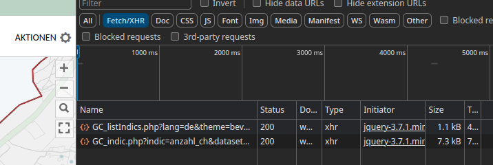
As you can see there is a listIndics and a indic API endpoint. ListIndics gives an overview of datasets, indic gives the data of the “indices”. Both require some specific payload to work, the most important being {‘lang’: ‘de’}. There is however a third endpoint that gives the crucial reference information, namely the name/id of the administrative feature at GC_refdata.php. Initially, I only used the indic endpoint to collect the data directly and the ref to get the reference frame. Combining requests to both, the data can be collected automatically, either to update or for the first time and come back in dict, including a headerline and meta information for the later export (also included above). Now you can get your up-to-date data from the Basler Atlas as well and have a better time using it for temporal analysis by running the above code and then calling this or something like this
data = get_basler_atlas(geographical_levels='block',themes={'bevstruk': ['alter0','alter20','alter65','w','m','gesbev'], },quiet=True)
This gives you the population data on the block level of the years from 1998 until today (2024 as of this writing). Calling the below saves the data to your home directory, namely 6 CSV files.
data2csv(data, outpath='~/')
Today I extended the code above to also get the available topics (i.e. the categories). Which allows us to discover topics or download data that would require some time to find otherwise.
geolevel ='block'for key, values in topics.items():if key !='bevstruk':continue data = get_basler_atlas(themes={key: values},quiet=True,geographical_levels=geolevel) of = data2csv(data, outpath='~/')break
As always, I hope this helps someone to discover data or save some time for themselves. And maybe at some point, I’ll find the time to document everything a bit better. Don’t forget to add the data source, i.e. the Stat. Amt Basel when you use their data.
Update/Fix
As I noticed today, there was some issue with the previous version of this script, namely a “deepcopy” issue that led to the fact, that the datacontainer had data from all connected subthemes when more than one was requested. Ups. But it should be fine now, the gist on top is updated and some usage information is added as well. 🙂
Make a map of the original and/or fixed coordinates of the hydrological stations of the BAFU using the data from Lindas
The above map is an illustration of the data we can extract with use of a SPARQL query and lindas of the hydrological data published on it. As you can see, there are two sets of points, one in Switzerland (corrected version) and one in the Mediterranean based on the “raw” lindas data (400km offset for some reason).
In my last post, I wanted to see how to get the current data of waterbodies from lindas.admin.ch in one table including geometry information. Now, we of course want to use Python to investigate the data; additionally, we want to extend our existing hydrodata SPARQL query to handle also a subset of stations instead of all stations.
import datetimeimport requestsimport pandas as pdimport numpy as npimport matplotlib.pyplot as plt# The prefixes, mainly to have them seperate PREFIXES="""PREFIX schema: <http://schema.org/>PREFIX hg: <http://rdf.histograph.io/>PREFIX la: <https://linked.art/ns/terms/>PREFIX ex: <http://example.org/># hydro related prefixesPREFIX h: <https://environment.ld.admin.ch/foen/hydro/>PREFIX hd: <https://environment.ld.admin.ch/foen/hydro/dimension/>PREFIX hgs: <https://environment.ld.admin.ch/foen/hydro/station/>PREFIX river: <https://environment.ld.admin.ch/foen/hydro/river/observation/>PREFIX lake: <https://environment.ld.admin.ch/foen/hydro/lake/observation/># geo related prefixesPREFIX wkt: <http://www.opengis.net/ont/geosparql#asWKT># hydrodata related prefixes (fake) that we use to reference to the historical data. haha.PREFIX hydrodata: <https://www.hydrodaten.admin.ch/plots/>"""## a function that makes the response to a dataframe, tailored to the hydrodata# and that also contains a small validation step to remove "outdated" valuesdef_response2dataframe(response,validate=True,time_threshold=datetime.timedelta(minutes=30)):# return pd.read_csv(io.StringIO(resp.text)) data = response.text.strip().split('\n') columns = data[0].split(',') data = [i.strip().split(',') for i in data[1:]] index = [i[0] for i in data] ix = columns.index('data') values = [[i[0]] + i[ix].split(';') for i in data] data = [[j for _, j inenumerate(i) if _ != ix]for i in data]# the dataframe holding all non measurement values columns.pop(ix) data1 = pd.DataFrame(columns=columns,data=data,index=index)for col in data1.columns: data1[col] = pd.to_numeric(data1[col], errors='ignore')def_list2dict(datalist):return {i: j for i, j inzip(datalist[::2], datalist[1::2])} values = {i[0]: _list2dict(i[1:])for i in values} ix = values.keys() columns = []for i in values.items(): vartypes =list(i[1].keys())for vartype in vartypes:if vartype in columns:passelse: columns.append(vartype) data = [[] for i in columns]for i in ix:for colno, colname inenumerate(columns): value = values[i][colname] if colname in values[i].keys() else'' data[colno].append(value) data = np.transpose(data) data2 = pd.DataFrame(columns=columns, data=data, index=ix)for col in data2.columns:if col !='measurementTime': data2[col] = pd.to_numeric(data2[col], errors='coerce') data = pd.concat([data1, data2], axis=1) data['query_time'] = pd.to_datetime(data['query_time']) data['measurementTime'] = pd.to_datetime(data['measurementTime'])if validate: time_threshold = pd.to_timedelta(time_threshold) good = data['query_time'] <= data['measurementTime'] + time_threshold# for illustration bad = data['query_time'] >= data['measurementTime'] + time_threshold data['measurementAge'] = data['query_time'] - data['measurementTime'] data = data[good]return datadefget_hydrodata(station_ids=None,return_as_dataframe=True,validate=True,time_threshold=datetime.timedelta(minutes=30)): query = ["""# what we want to get out of the query as "nicely" formatted data SELECT ?station_id ?station_name ?station_type ?station_type_nice ?latitude ?longitude ?station_iri ?station_data_iri ?station_geometry_iri (group_concat(?measurement_type_measurement_value;SEPARATOR=";") as ?data) ?query_time # add the https://hydrodaten.admin.ch url for the data that go back 7 days (actually 40 days sometimes, see dev console) (if(contains(?data,"discharge"), uri(concat(str(hydrodata:), 'p_q_7days/', ?station_id, '_p_q_7days_de.json')), "") as ?hydrodata_url_discharge_waterlevel) (if(contains(?data,"temp"), uri(concat(str(hydrodata:), 'temperature_7days/', ?station_id, '_temperature_7days_de.json')), "") as ?hydrodata_url_temperature)"""# where part including initial setup of measurement types""" WHERE { ?station ?prop ?value. filter( ?prop in (ex:isLiter, hd:measurementTime, hd:waterTemperature, hd:waterLevel, hd:discharge))""",# generating data and variables part""" bind(replace(replace( str(?station), str(river:), "", "i"), str(lake:), "", "i") as ?station_id) # the above is equivalent to this in theory but the above uses prefixes so would be easier to change # in case of changes # bind(strafter(str(?station), "observation/") as ?station_id2) # get the kind of station this is (whether lake or river) - the hierarchy/ontology here is weird as all are measurement stations # or observation but the distinction is river/lake first then observation bind(strbefore(strafter(str(?station), str(h:)), "/") as ?station_type) # uppercase the first letter -> why is there no capitalize function in SPARQL :throw_table: bind(concat(ucase(substr(?station_type,1,1)), substr(?station_type,2,strlen(?station_type)-1)) as ?station_type_nice) # remove some filler words from the data bind(replace(str(?prop), str(hd:), "", "i") as ?measurement_type) # convert the actual measurement value to a literal bind(str(?value) as ?measurement_value) # introduce the time of the query to (maybe) see if the values are old bind( str(now()) as ?query_time) # combine the type of measurement with the value so we can group by and not loose information bind(concat(?measurement_type, ';', ?measurement_value, '') as ?measurement_type_measurement_value) # start making IRIs so we can check/link back to lindas # the IRI containing information of the station itself (not linked to river/lake) bind(IRI(concat(str(hgs:), ?station_id)) as ?station_iri) # generate the geometry IRI bind(IRI(concat(str(hgs:), concat(?station_id,"/geometry"))) as ?station_geometry_iri) # generate the station IRI that holds the data information bind(IRI(concat(str(h:), ?station_type, "/observation/", ?station_id)) as ?station_data_iri) # get the information about the location of the station ?station_geometry_iri wkt: ?coordinates. # also get the name ?station_iri schema:name ?stat_name. bind(replace(?stat_name, ',', ';') as ?station_name) # simplifiy the geometry to lon/lat in array form BIND(STRBEFORE(STRAFTER(STR(?coordinates), " "), ")") AS ?latitude) BIND(STRBEFORE(STRAFTER(STR(?coordinates), "("), " ") AS ?longitude) }""",# grouping part""" group by # the station information ?station_id ?station_type ?station_type_nice ?station_name ?latitude ?longitude # the IRIs ?station_iri ?station_data_iri ?station_geometry_iri # validation information ?query_time""",# sorting part""" order by ?station_id""" ]if station_ids isnotNone:# per default, get all stations but if some stations are given uses# this modication instead station_ids = station_ids ifisinstance( station_ids, list) elselist(station_ids) station_ids ='"'+'","'.join([str(i) for i in station_ids]) +'"' query.insert(1, f'filter (?station_id in ({station_ids}))') query =PREFIXES+'\n'.join(query) resp = requests.post("https://ld.admin.ch/query",data="query="+ query,headers={"Content-Type": "application/x-www-form-urlencoded; charset=utf-8","Accept": "text/csv" } ) resp.encoding ="utf-8"if return_as_dataframe: resp = _response2dataframe(resp,validate=validate,time_threshold=time_threshold)return resp, queryif__name__=='__main__': df, query = get_hydrodata() subset = [2091, 2613] df_subset, query_subset = get_hydrodata(station_ids=subset,return_as_dataframe=True)
A first approach is given by the lindas help which showcases the use of the typical request together with pandas. The example is straightforward but not usually how we’ll have data (more than 3 columns ..) that are useful with pandas. As we’ve seen in the last exploration of lindas, we can write a query that gives us a row for each station of the hydrological network of the BAFU. To be consistent with the example, we want a CSV return, which means replacing all commas with something better (especially the names of stations sometimes do have a comma inside). Other than that, the query that we used before also works directly via Python and we only extended it with the option to additionally filter with station_ids by adding the below (which adds a very simple filter into the query):
if station_ids isnotNone:# per default, get all stations but if some stations are given uses# this modication instead station_ids = station_ids ifisinstance( station_ids, list) elselist(station_ids) station_ids ='"'+'","'.join([str(i) for i in station_ids]) +'"' query.insert(1, f'filter (?station_id in ({station_ids}))')
Additionally, as I didn’t manage to split the values again into separate columns after the grouping (or only with a lot of needless wordiness), I wrote a small converter function that mainly extracts the general information (meta-information if you will like latitude/longitude or similar) and converts the actual measurement data into columns and concatenates the two.
## a function that makes the response to a dataframe, tailored to the hydrodata# and that also contains a small validation step to remove "outdated" valuesdef_response2dataframe(response,validate=True,time_threshold=datetime.timedelta(minutes=30)):# return pd.read_csv(io.StringIO(resp.text)) data = response.text.strip().split('\n') columns = data[0].split(',') data = [i.strip().split(',') for i in data[1:]] index = [i[0] for i in data] ix = columns.index('data') values = [[i[0]] + i[ix].split(';') for i in data] data = [[j for _, j inenumerate(i) if _ != ix]for i in data]# the dataframe holding all non measurement values columns.pop(ix) data1 = pd.DataFrame(columns=columns,data=data,index=index)for col in data1.columns: data1[col] = pd.to_numeric(data1[col], errors='ignore')def_list2dict(datalist):return {i: j for i, j inzip(datalist[::2], datalist[1::2])} values = {i[0]: _list2dict(i[1:])for i in values} ix = values.keys() columns = []for i in values.items(): vartypes =list(i[1].keys())for vartype in vartypes:if vartype in columns:passelse: columns.append(vartype) data = [[] for i in columns]for i in ix:for colno, colname inenumerate(columns): value = values[i][colname] if colname in values[i].keys() else'' data[colno].append(value) data = np.transpose(data) data2 = pd.DataFrame(columns=columns, data=data, index=ix)for col in data2.columns:if col !='measurementTime': data2[col] = pd.to_numeric(data2[col], errors='coerce') data = pd.concat([data1, data2], axis=1) data['query_time'] = pd.to_datetime(data['query_time']) data['measurementTime'] = pd.to_datetime(data['measurementTime'])if validate: time_threshold = pd.to_timedelta(time_threshold) good = data['query_time'] <= data['measurementTime'] + time_threshold# for illustration bad = data['query_time'] >= data['measurementTime'] + time_threshold data['measurementAge'] = data['query_time'] - data['measurementTime'] data = data[good]return data
Additionally, we can fix the offset that we found (~400 km in latitude) in the geometry by using the following (after importing my conversion functions):
Now we can see the difference, especially when we plot the dataframe of water temperatures (the labelling is really overkill at this point and just for illustration):
## fix the offsethw, rw = wgs84_to_ch1903(df['latitude'], df['longitude'], plus=True)hw = hw +400000lat, lon = ch1903_to_wgs84(hw, rw)# setup the mapimport cartopy.crs as ccrsimport cartopy.feature as cffig, ax = plt.subplots(dpi=200, figsize=[9, 9], subplot_kw={"projection":ccrs.PlateCarree()})thevar ='waterTemperature'units = {'waterLevel': 'm MSL', 'waterTemperature': '°C', 'discharge': 'm³/s'}# show the "original" coordinatess = ax.scatter(df['longitude'], df['latitude'], s=150, edgecolor='k', c=df[thevar], vmin=0, vmax=25, cmap='coolwarm')# show the fixed coordinatess = ax.scatter(lon, lat, s=150, edgecolor='k', c=df[thevar], cmap='coolwarm', vmin=0, vmax=25)# the respective name of the station as label if need beadd_station_label =Falseif add_station_label:for sid, thevalue, lon, lat, station_name inzip(df['station_id'], df[thevar], df['longitude'], df['latitude'], df['station_name']):if np.isnan(thevalue):continue ax.text(lon, lat, station_name.replace(';','\n').replace('','\n'), va='center', ha='center', fontsize=3, clip_on=True)# map decorationsax.set_xlabel('Longitude (°)')ax.set_ylabel('Latitude (°)')plt.colorbar(s, aspect=50, pad=0.1, location='bottom', label=f'{thevar.replace("water","").capitalize()}'+f' ({units[thevar]})')ax.set_title(f'Hydrodata in Switzerland')ax.gridlines(draw_labels=True, dms=True, x_inline=False, y_inline=False, lw=0.25, color='k')# if you want, add a stockimage but it won't look nice at this resolution#ax.stock_img()# add coastline and borders to illustrateax.coastlines()ax.add_feature(cf.BORDERS)# set proper boundaries for illustrationax.set_ylim(42, 48)ax.set_xlim(5, 12)
If you wish instead to only plot data points that have a valid temperature you can use the condition notnull() on the variable:
# fix the offsethw, rw = wgs84_to_ch1903(df['latitude'], df['longitude'], plus=True)hw = hw +400000lat, lon = ch1903_to_wgs84(hw, rw)# setup the mapfig, ax = plt.subplots(dpi=200, figsize=[16, 12], subplot_kw={"projection":ccrs.PlateCarree()})thevar ='waterTemperature'units = {'waterLevel': 'm MSL', 'waterTemperature': '°C', 'discharge': 'm³/s'}# filter out stations without values for this variablecond = df[thevar].notnull()# show the "original" coordinatess = ax.scatter(df['longitude'][cond], df['latitude'][cond], s=150, edgecolor='k', c=df[thevar][cond], vmin=0, vmax=25, cmap='coolwarm')# show the fixed coordinatess = ax.scatter(lon[cond], lat[cond], s=150, edgecolor='k', c=df[thevar][cond], cmap='coolwarm', vmin=0, vmax=25)# map decorationsax.set_xlabel('Longitude (°)')ax.set_ylabel('Latitude (°)')plt.colorbar(s, aspect=50, pad=0.1, location='bottom', label=f'{thevar.replace("water","").capitalize()}'+f' ({units[thevar]})')ax.set_title(f'Hydrodata of Switzerland')ax.gridlines(draw_labels=True, dms=True, x_inline=False, y_inline=False, lw=0.25, color='k')# if you want, add a stockimage but it won't look nice at this resolution#ax.stock_img()# add coastline and borders to illustrateax.coastlines()ax.add_feature(cf.BORDERS)# set proper boundaries for illustrationax.set_ylim(45.5, 48)ax.set_xlim(5.5, 11)
Going forward, you could use requests to download the past measurement data that are linked in the dataframe via the query (hydrodata URL) and make an animation; probably xarray would be a better choice for holding the data then though…
Hope this was interesting on how to combine and going forward we’ll look at using openlayers and the JSON response from lindas to make a map.
PS: On another note, while we found an offset last time, there is one station in the dataset that has a wrong longitude as well, the station with id 2270 “Combe des Sarrasins” with latitude of 41.315… and longitude of 0.296… according to its lindas entry but should really be at 47.195… , 6.877…